Modeling RTS

What is Random Telegraph Signal?

The transistor technology in a CMOS detector is typically a field effect transistor (FET), which converts photons to charge in the pixel itself. Those transistors have very thin layers of semiconductor material (intentionally so) with very low operating currents. However, lattice defects can have a significant effect on the voltage to current transformation in those FETs. A well-documented phenomenon of FET transistors is random telegraph noise (RTN), where the measured drain current fluctuates in time among N discrete levels for a constant gate voltage. This fluctuation is driven by lattice defects. Typically there are 2 discrete levels, but more states can be present in a given MOSFET.

"Data variation of an RTS affected pixel, showing three different modes of clustering"

The conversion from charge to voltage (or, a digital number) is typically achieved with correlated double sampling (CDS), where the pixel output level is measured as the difference between a reset level and the pixel signal (charge) level. The advantage of CDS is that it reduces temporal variations in the offset level of the amplifiers, i.e., it adresses 1/f noise. CDS is also used in CCD detectors, and in both detector types, the output signal is reported as the difference between two measurements.

In CMOS detectors, CDS is complicated by the fact that each of the two readouts might have one of the two discrete responses to an input level due to RTN: The effect of those two readout levels can either cancel out in CDS (i.e., both reset and signal level were measured in the same RTN state), or systematically shift the result of CDS higher or lower if the reset and signal measurement had different RTN states. This in effect leads to a trimodal distribution of output level for the same input signal level.

"A histogram of the RTS affected pixel, showing a trimodal distribution"

Gaussian Mixture Models and RTS Properties

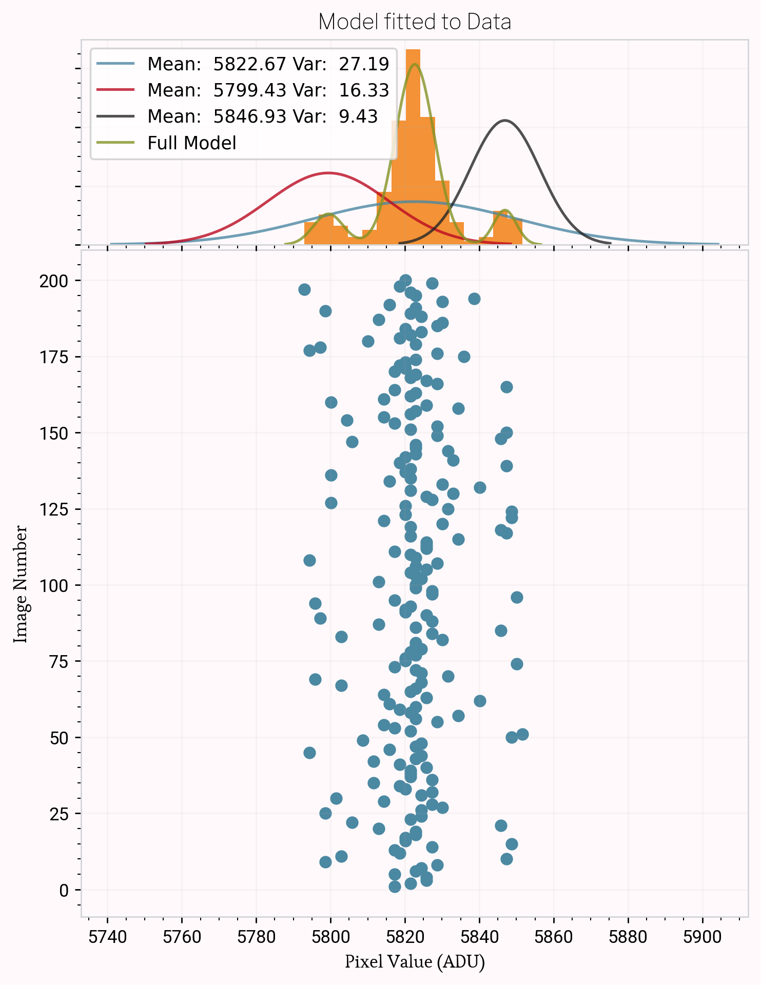
As we plotted histograms for the pixels on a detector, we found unimodal, bimodal, and trimodal pixel noise distributions. Our end goal was to parametrize the noise by finding the peak locations and variances for each peak present. After some trial and error with Maximum Likelihood fitting and Kernel Density Estimation on the histograms, Gaussian Mixture Modelling seemed to be the best option to non-parametrically model the data (not the histogram representation of it).

Gaussian Mixture Model Basics

Gaussian Mixture Modelling is a parametric probability density function represented as a weighted sum of Gaussian component densities. It attempts to represent the data as a sum of weighted gaussians with unique means, and covariances:

\[p( \textbf{x}| \lambda ) = \sum_{i=1}^{M} w_{i} g(\textbf{x}| \mu_{i} \Sigma_{i} )\]

After determining the number of components in the data, the parameters are estimated from the data by the iterative Expectation-Maximization algorithm. We use sklearn to implement this modelling method in our code.

A difficult part of this implementation is determining the number of components needed to model the data. This changes for each pixel, so we wanted an automated way to determine this, without overfitting.

The primary method we use to do this is a silhouette score. This is calculated by the GMM class provided by sklearn, and is a simple calculation.
For a given sample, the likelihood that it belings to a cluster is determined by:

\[s = \frac{b-a}{max(a,b)}\]

"A visual representation of a silhouette score, a represents intra-cluster distance from the sample, and b is the inter-cluster distance."

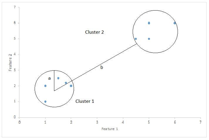
Where, a represents intra-cluster distance from the sample, and b is the inter-cluster distance. Source: Bhardwaj, 2020

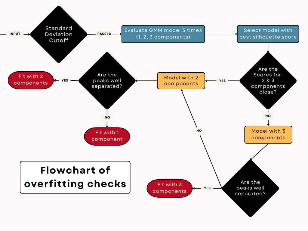
Then to avoid overfitting, we go through a series of checks illustrated below:

"A flowchart depciting the checks made to ensure the right number of components are fitted to the data. THe checks include ones of peak separation, and silhouette scores."

At the end, we get parameters describing the data:

peak_location : TYPE: list(float), length = num_peaks
    DESCRIPTION: The means of each of the Gaussian modes calculated by GMM
peak_widths : TYPE: list(float), length = num_peaks
    DESCRIPTION: The covariance of each Gaussian mode calculated by GMM
num_peaks : TYPE: int
    DESCRIPTION: The number of Gaussians used to model the distribution of values of the pixel
amp : TYPE: list(float)
    DESCRIPTION: The weights of each gaussian in the mixture. All weights sum to 1.

"The model, histogram, and data of an RTS affected pixel with three modes."

"The model, histogram, and data of an RTS affected pixel with two modes."

RTS Properties

After modelling a subset of 500x500 pixels in each image in the test data (200 bias frames taken with a QHY411 CMOS camera), we can investigate the properties of the pixels affected by telegraph noise. In doing so, we find the following:

7.8% of examined pixels are multimodal.
The locations are consistent.
Majority of pixels are trimodal; though unexpectedly, a small number of pixels have a bimodal distribution.
When run on all pixels in a 500x500 pixel grid, 12% of pixels are affected
73% of RTS pixels neighbor another RTS pixel.

"A map of locations of bad pixels, color coded by modality. There is a zoomed in section in the top left corner of the map showing adjacency of trimodal."

Impact on Astronomical Images

CMOS cameras are not that widely used in astronomy yet, and we want to understand if CMOS peculiarities require seem special treatment in the data processing software. We note:

The max telegraph noise amplitude of 20e- as seen in the QHY411 is still not relevant for well-exposed stars, as for exposure levels >20e-^2 one would be dominated by shot noise.
Telegraph noise could have an important impact on for low light level sources and precise background estimation.
In particular in undersampled situations, one would watch out for the additional impact of telegraph noise on a single measurement.
Telegraph noise might be most important to treat in calibration images such as bias and darks, as those propagate to all calibrated images.
When binning data, which is an entire software process in COS cameras post-readout, it might be beneficial to initially preserve the full data and then be more sophisticated in binned to flat / exclude/treat high RTN pixels.
Also, as we go to a more sophisticated noise propagation in the data processing, a more sophisticated per-pixel noise description may be useful.

Error Propagation

With the means, amplitudes, and covariances of individual gaussians we can follow standard error propagation methods to calculate the read noise of each pixel. This is possible because our model essentially models the probability distribution function of the data.

To get from covariance to a variance of each of our 1D gaussians:

\[\sigma_{i}^{2} = Tr(\Sigma_i)\]

And then for multiple components, we can propagate the parameters to get a single read nosie for a pixel.

\[\sigma^2 = \sum_{i} w_{i} \sigma_{i}^{2} + \sum_{i} w_{i} \left( \mu_{i} \right)^{2} - \left( \sum_{i} w_{i} \mu_{i} \right)^2\]

where the read noise is the square root of sigma.